Eggbox

This example will explore the classic eggbox function using Models.Eggbox.

Setup

For this example, you'll need to add the following packages

julia>]add Distributions MCMCChains Measurements NestedSamplers StatsBase StatsPlots

Define model

using NestedSamplers

model, logz = Models.Eggbox()

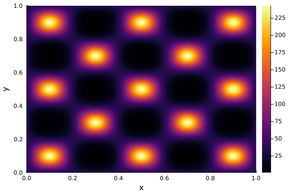
let's take a look at a couple of parameters to see what the log-likelihood surface looks like

using StatsPlots

x = range(0, 1, length=1000)
y = range(0, 1, length=1000)
loglike = model.prior_transform_and_loglikelihood.loglikelihood
logf = [loglike([xi, yi]) for yi in y, xi in x]
heatmap(
    x, y, logf,
    xlims=extrema(x),
    ylims=extrema(y),
    xlabel="x",
    ylabel="y",
)

Sample

using MCMCChains
using StatsBase
# using multi-ellipsoid for bounds
# using default rejection sampler for proposals
sampler = Nested(2, 500)
chain, state = sample(model, sampler; dlogz=0.01, param_names=["x", "y"])
# resample chain using statistical weights
chain_resampled = sample(chain, Weights(vec(chain[:weights])), length(chain));

Results

chain_resampled

Chains MCMC chain (6333×3×1 Array{Float64, 3}):

Iterations        = 1:6333
Number of chains  = 1
Samples per chain = 6333
parameters        = x, y
internals         = weights

Use `describe(chains)` for summary statistics and quantiles.

marginalkde(chain[:x], chain[:y])
plot!(xlims=(0, 1), ylims=(0, 1), sp=2)
plot!(xlims=(0, 1), sp=1)
plot!(ylims=(0, 1), sp=3)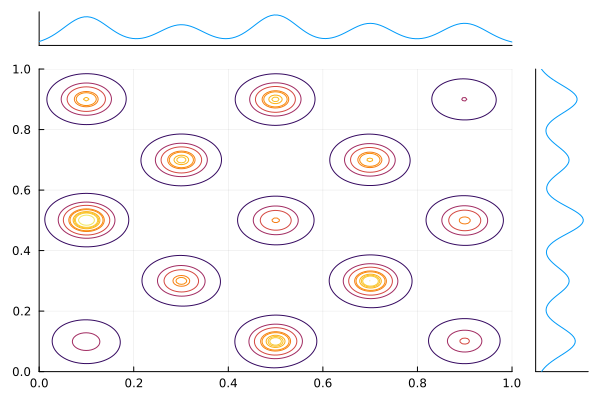

density(chain_resampled, xlims=(0, 1))
vline!(0.1:0.2:0.9, c=:black, ls=:dash, sp=1)
vline!(0.1:0.2:0.9, c=:black, ls=:dash, sp=2)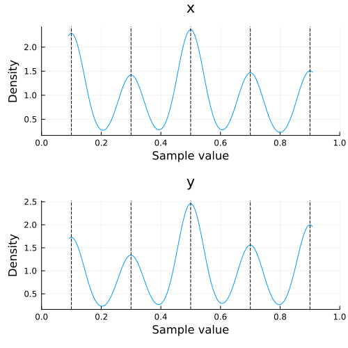

using Measurements
logz_est = state.logz ± state.logzerr
diff = logz_est - logz
println("logz: $logz")
println("estimate: $logz_est")
println("diff: $diff")

logz: 235.88
estimate: 235.94 ± 0.11
diff: 0.065 ± 0.11