Correlated Gaussian

This example will explore a highly-correlated Gaussian using Models.CorrelatedGaussian. This model uses a conjuage Gaussian prior, see the docstring for the mathematical definition.

Setup

For this example, you'll need to add the following packages

julia>]add Distributions MCMCChains Measurements NestedSamplers StatsBase StatsPlots

Define model

using NestedSamplers

# set up a 4-dimensional Gaussian
D = 4
model, logz = Models.CorrelatedGaussian(D)

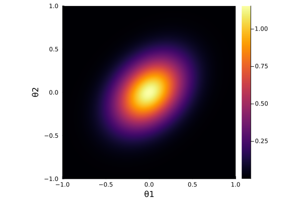
let's take a look at a couple of parameters to see what the likelihood surface looks like

using StatsPlots

θ1 = range(-1, 1, length=1000)
θ2 = range(-1, 1, length=1000)
loglike = model.prior_transform_and_loglikelihood.loglikelihood
logf = [loglike([t1, t2, 0, 0]) for t2 in θ2, t1 in θ1]
heatmap(
    θ1, θ2, exp.(logf),
    aspect_ratio=1,
    xlims=extrema(θ1),
    ylims=extrema(θ2),
    xlabel="θ1",
    ylabel="θ2"
)

Sample

using MCMCChains
using StatsBase
# using single Ellipsoid for bounds
# using Gibbs-style slicing for proposing new points
sampler = Nested(D, 50D;
    bounds=Bounds.Ellipsoid,
    proposal=Proposals.Slice()
)
names = ["θ_$i" for i in 1:D]
chain, state = sample(model, sampler; dlogz=0.01, param_names=names)
# resample chain using statistical weights
chain_resampled = sample(chain, Weights(vec(chain[:weights])), length(chain));

Results

chain_resampled

Chains MCMC chain (2350×5×1 Array{Float64, 3}):

Iterations        = 1:2350
Number of chains  = 1
Samples per chain = 2350
parameters        = θ_1, θ_2, θ_3, θ_4
internals         = weights

Use `describe(chains)` for summary statistics and quantiles.

corner(chain_resampled)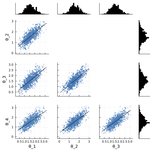

using Measurements
logz_est = state.logz ± state.logzerr
diff = logz_est - logz
println("logz: $logz")
println("estimate: $logz_est")
println("diff: $diff")

logz: -6.187913267630009
estimate: -6.21 ± 0.13
diff: -0.019 ± 0.13